Logistic regression
Logistic regression is used to model a binary response variable in terms of explanatory variables.
An example
The data for this example are based on data collected by the Department of Agriculture as part of their routine screening of airline passengers arriving in Australia. The original data, which are confidential, were used to guide the construction of this dataset.
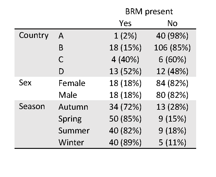
The data are 200 passenger arrivals from 2013 and 2014. The outcome of interest is whether or not the airline passenger was carrying material considered to pose a biosecurity risk. Common biosecurity risk material (‘BRM’) includes animal products, fresh fruit and seeds. In our data, 18% of passengers arriving were found to be carrying BRM. For each arrival, various passenger and travel characteristics are provided. For the purposes of this example we will consider the passport country of the passenger, their sex, their historical number of trips, and the season of their arrival. Note that the passport country has been deliberately anonymised.
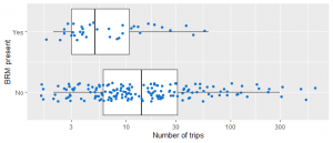
The following table and figure give a summary of the relationship between the presence of BRM and each of these characteristics (our explanatory variables). The number of trips has been transformed using a log10 transformation in the boxplot to aid visual interpretation.
An appropriate report of a logistic regression analysis may include this kind of information before the results of the formal analyses are given.
The report of the analysis itself will usually include overall tests for the explanatory variables included in the model, along with estimated odds ratios from the model. Often the results are presented as both unadjusted (or crude) odds ratios based on a simple model with only one variable at a time, and adjusted odds ratios for a model with all the variables, to help unpack how the adjustment affects the impact of a particular explanatory variable. For categorical variables, a reference group is needed for these odds ratios, and ought to be clearly specified in any tables. For numerical variables, the odds ratio is usually for a change of one unit in the variable but other size changes may be presented.
Examples of these are below.

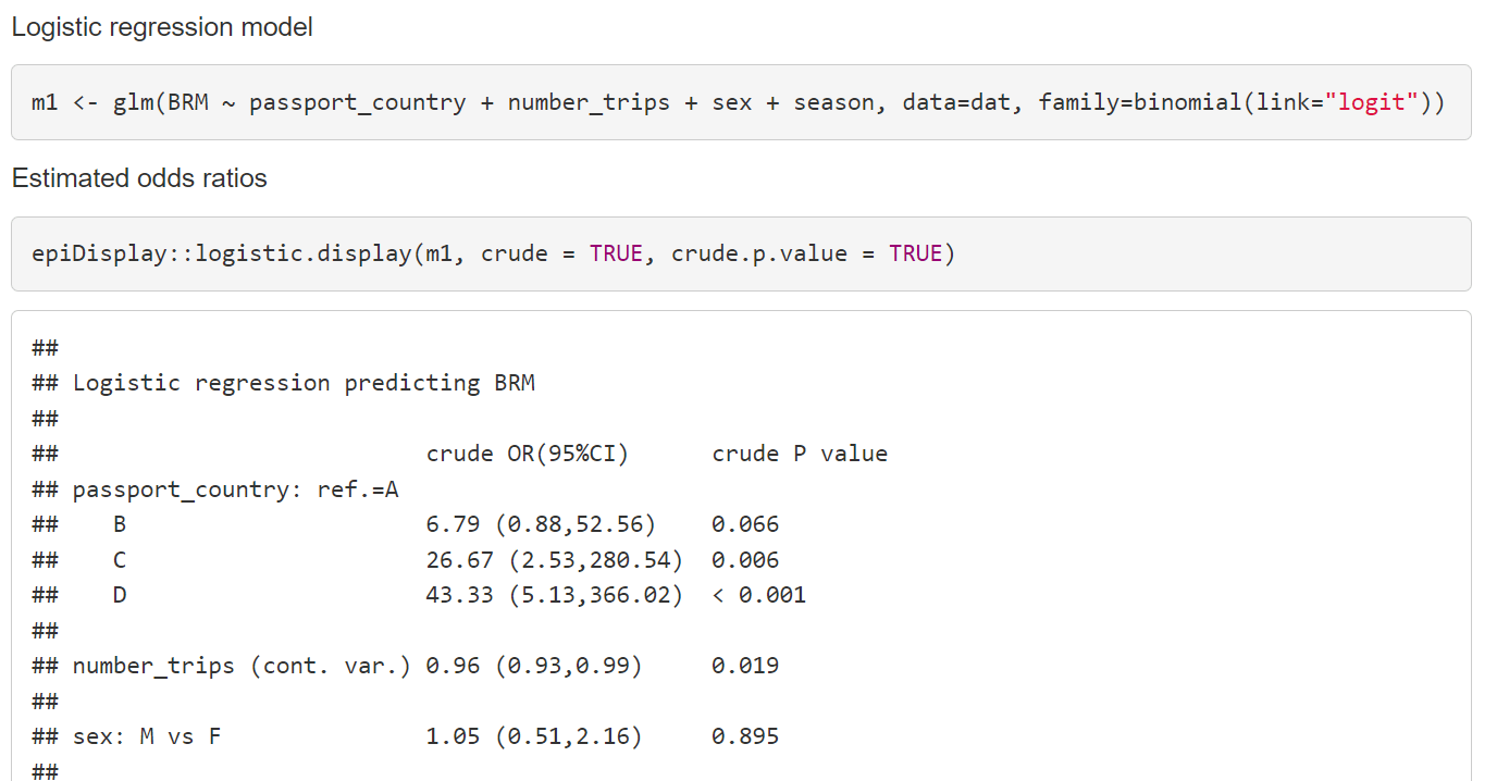
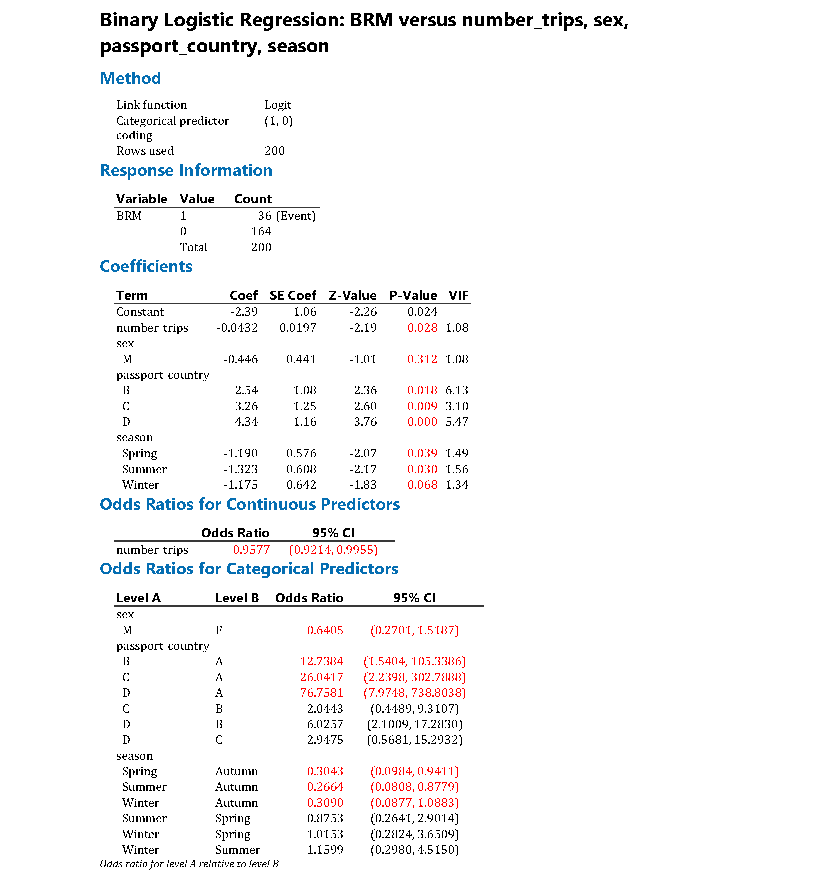
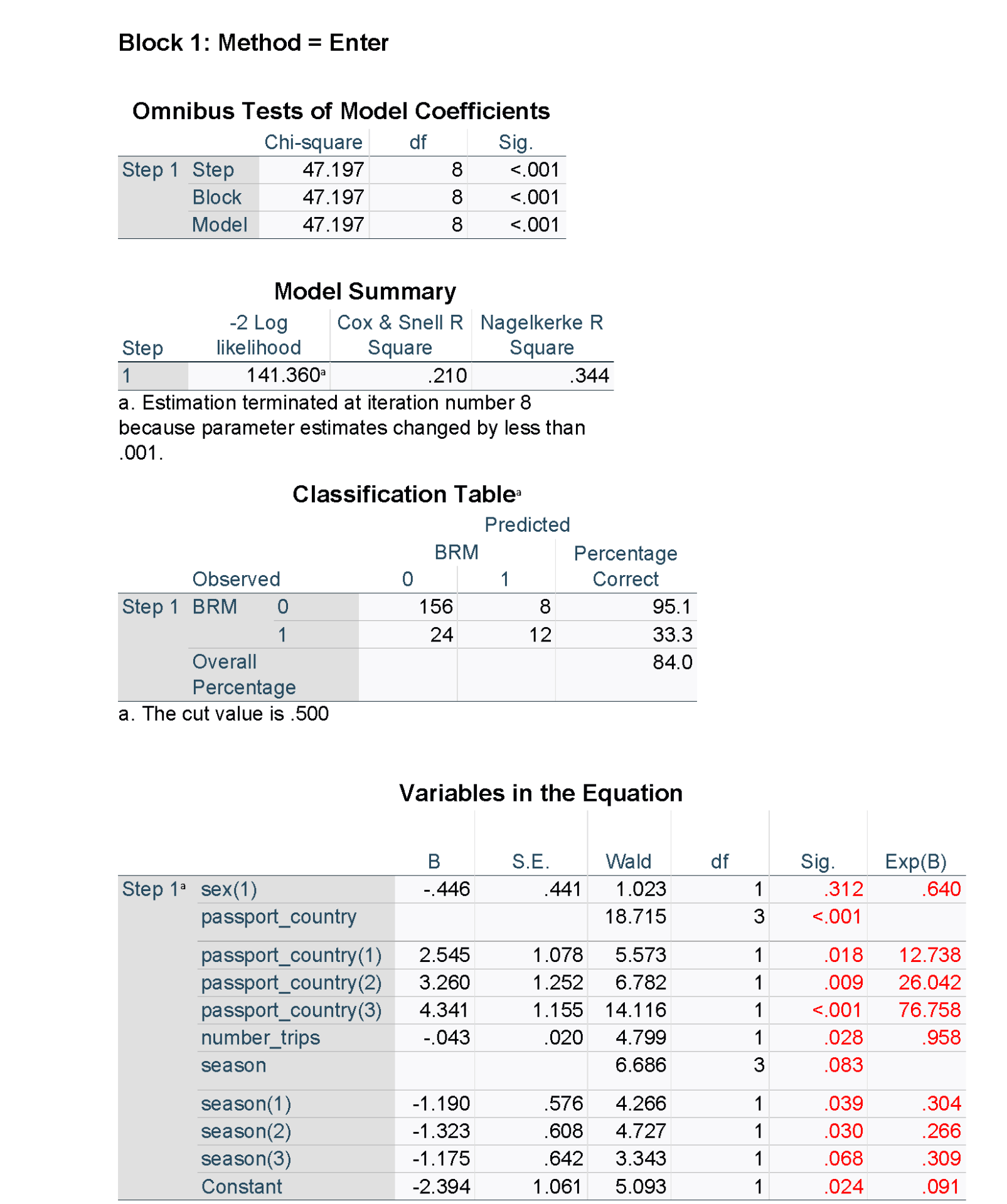
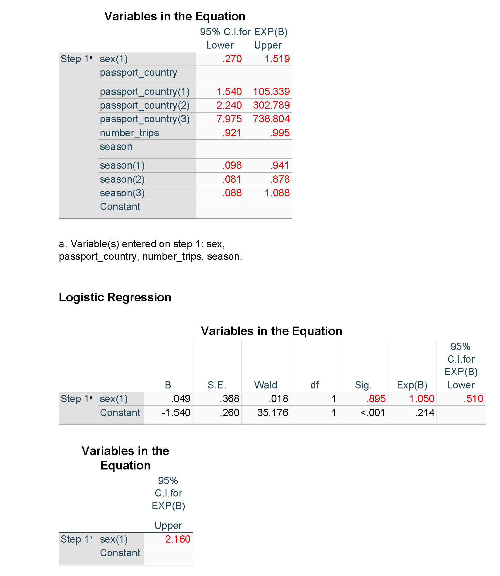
It can be helpful to describe at least some of the relationships in words in order to aid correct interpretation of the odds ratios. For example, the passport country of the passenger was found to be strongly related to the odds of being found to be carrying BRM (in this case, likely due to the variation in border practices of different countries). Consider Country A vs Country B. As the results above indicate, after adjusting for other factors, we estimate that the odds of a passenger from Country B found to be carrying BRM are 12.7 times higher than for a passenger from Country A. We are 95% confident that the true odds ratio is between 1.54 and 105; this is a wide interval, but nevertheless evidence of a strong association. Similarly, for each additional trip a passenger has taken, their odds of being found to be carrying BRM are estimated to decrease by a factor of 0.96 (or by 4%), after adjusting for the other factors. This can also be described for a different interval or scale, for example, for every five additional trips that a passenger has taken, their odds of being found to be carrying BRM are estimated to decrease by a factor of 0.82 (or by 18%).
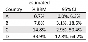
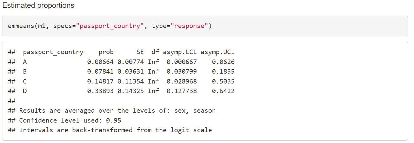
Sometimes it is useful to present the outcome as estimated proportions or percentages across the levels of a categorical variable. Note that this has to be calculated for fixed levels of the other explanatory variables, typically means of the continuous variables and the average of the result across all the combinations of the levels of the categorical variables. The following table gives the estimated percentage of arrivals with BRM for each country (a key explanatory variable), along with a 95% confidence interval.
The following demonstrates the kind of output you can expect from various statistical software packages for a logistic regression model.
R
The output in R is shown below; RMarkdown has been used to produce this output.

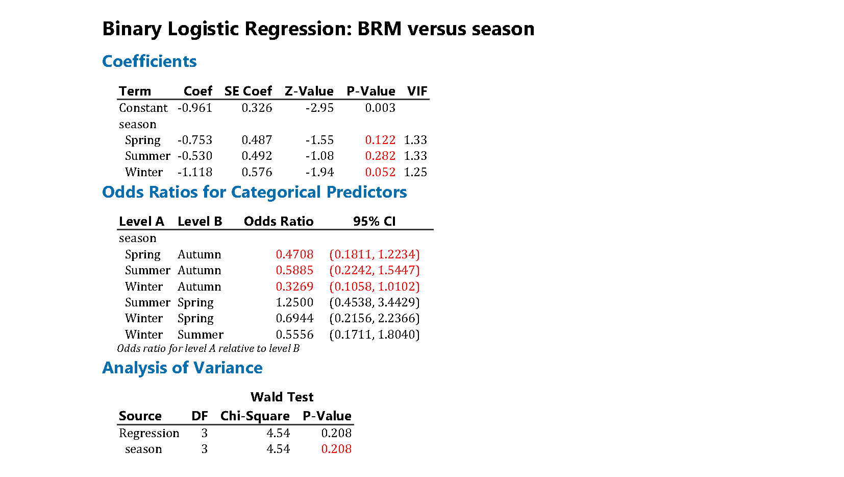
Minitab
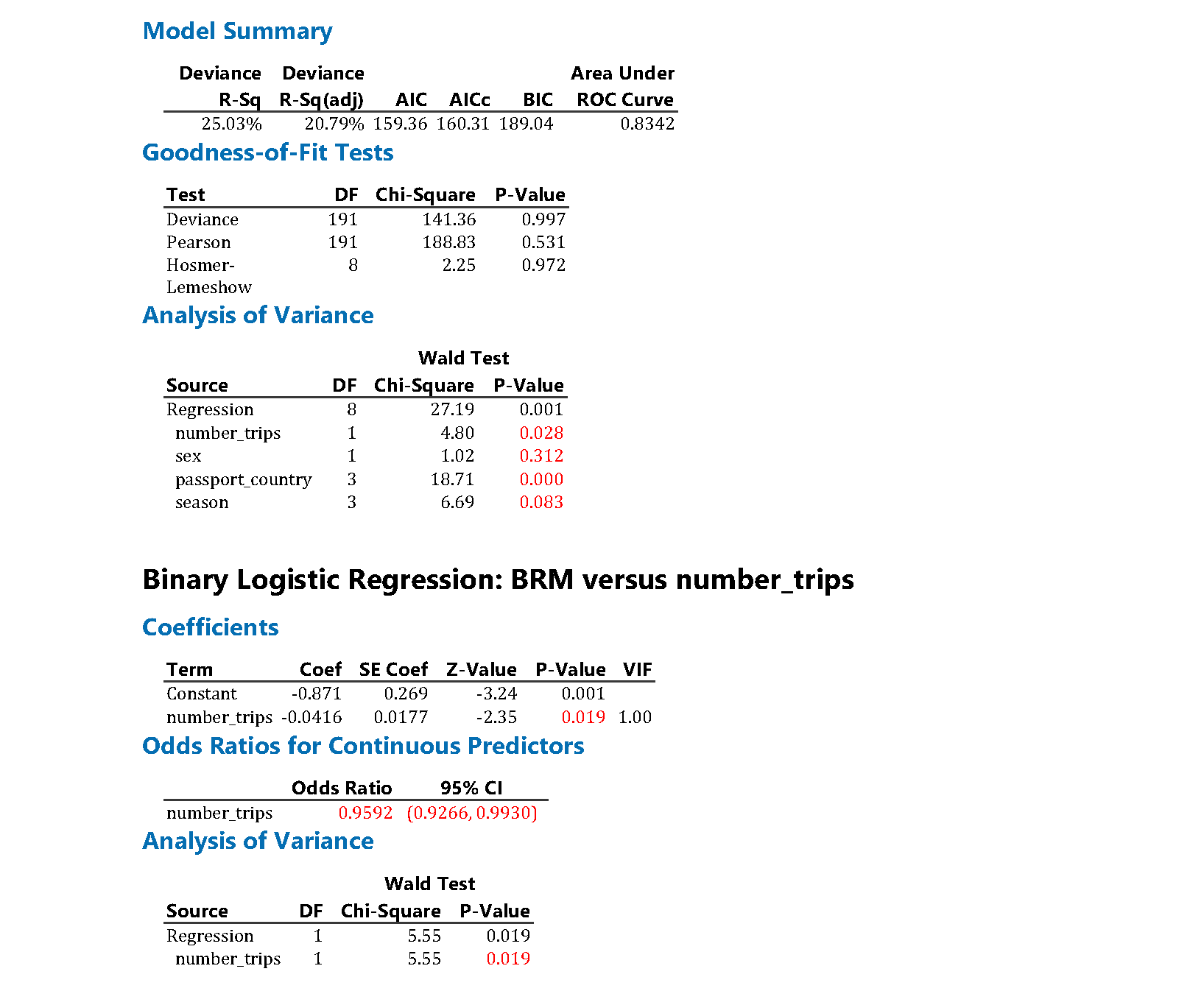
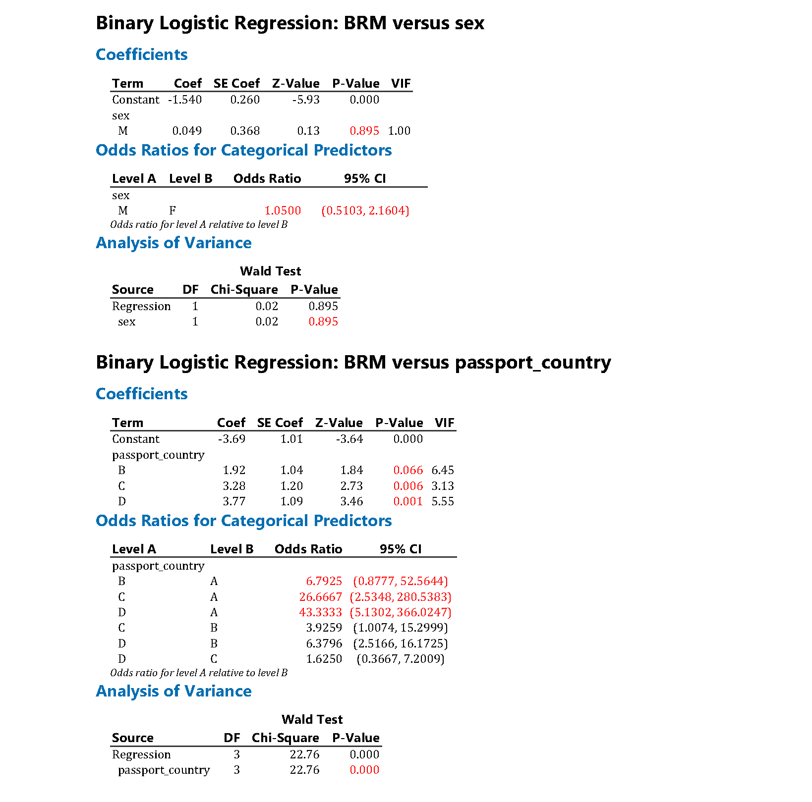
The output from Minitab is shown below. Note that some of the results for the unadjusted models have been suppressed for clarity, and figures used in the tables have been highlighted in red. Unlike R and the emmeans package, the estimated percentages averaged over the other explanatory variables are not available directly in Minitab, but estimates can be obtained for a given set of values of the explanatory variables.
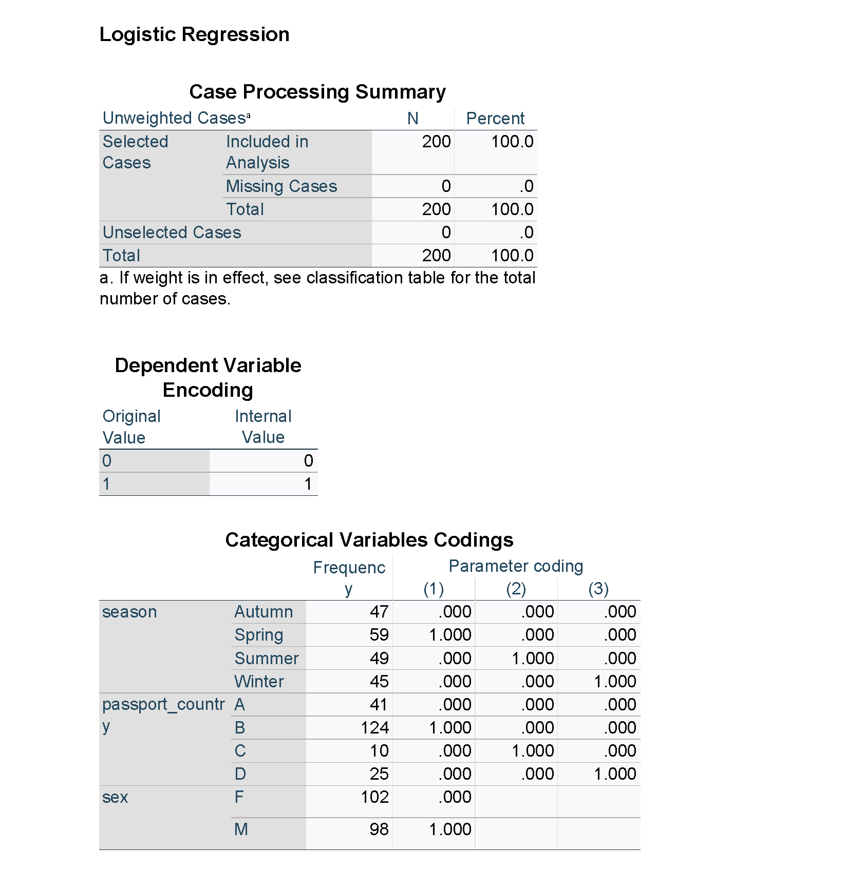
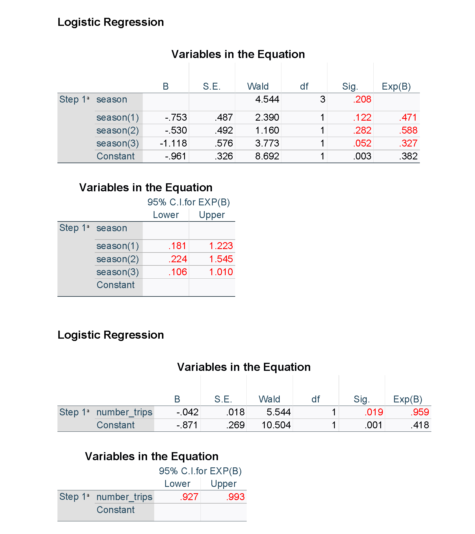
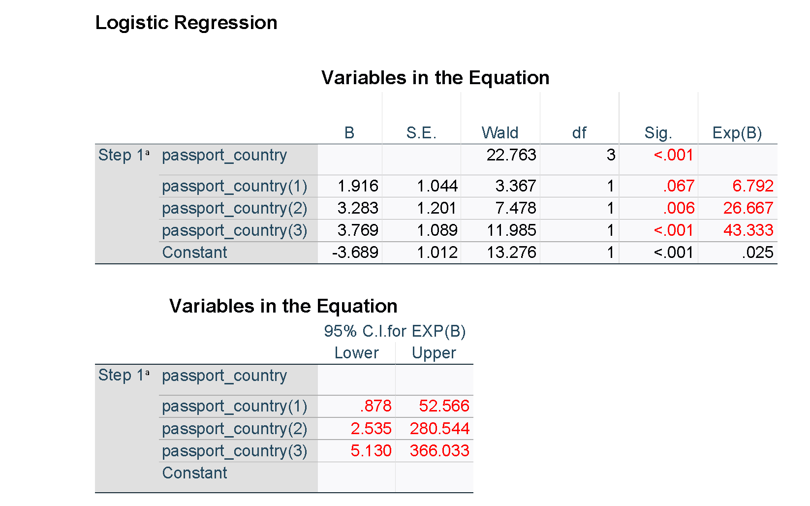
SPSS
The output from SPSS is shown below. Note that some of the results for the unadjusted models have been suppressed for clarity, and figures used in the tables have been highlighted in red. Unlike R and the emmeans package, the estimated percentages averaged over the other explanatory variables are not available directly in SPSS, but predicted percentages can be obtained for each of the observations in the data set.
Categories
- Uncategorised