Independent samples t-test and confidence interval for the difference of means
An example
The data for this example come a remarkable experiment carried out in the Department of Zoology at the University of Melbourne, over 22 years, by Wilfred Agar, Frank Drummond, Oscar Tiegs and Mary Gunson. The experiment was a test of the theory of Lamarckian inheritance, which states that offspring can inherit characteristics that are acquired or learnt by their parents during the parents’ lifetime. They tested the idea out by testing 50 generations of rats; rats in one group were trained on a learning task over the generations whereas the other group was not. The rats had to learn to escape from a tank of water from one of two exits. The correct exit was dimly lit whereas the wrong exit was brightly lit. The bright exit was “wrong” because an electric shock was given at this exit. The intention was to induce a phobia of bright lights.
The data for each generation are published, but here were consider the number of errors made by the rats in the 14th generation; there were 37 control rats and 50 trained rats in this generation. There are results for two groups of different rats to compare, so the design involves two independent groups. As the number of errors is a quantitative variable, the methods of statistical inference that can be applied here usually found under labels such as “2-sample t-test” or “independent samples t-test” in software menus or code.
An appropriate report of the analysis may include summary statistics, the estimated difference of means with a 95% confidence interval, and a P-value. The P-value is for a test of the null hypothesis of no difference in the true means of the two groups.
Here is a summary table that combines descriptive and inferential statistics. It uses the results from the analysis that does not assume equal variances.

This layout will allow you to add more rows with results from different outcomes, if you need. There are, of course, other ways of producing good summary tables for this analysis.
SPSS
The statistics that are included in the summary table above are highlighted in red in this SPSS output. Note that values have to rounded and that the P-value is labelled appropriately in the summary table. In some disciplines, you are also required to report the test statistic. The relevant information from the SPSS output is highlighted in blue. You could add a column to the table to report the test statistic: t(78.7) = 1.89.
| Group Statistics | |||||
| Group | N | Mean | Std. Deviation | Std. Error Mean | |
| Number of errors | Control | 37 | 19.351 | 12.4303 | 2.0435 |
| Trained | 50 | 14.200 | 12.7167 | 1.7984 | |
| Independent Samples Test | ||||||||||
| Levene’s Test for Equality of Variances | t-test for Equality of Means | |||||||||
| F | Sig. | t | df | Sig. (2-tailed) | Mean Difference | Std. Error Difference | 95% Confidence Interval of the Difference | |||
| Lower | Upper | |||||||||
| Number of errors | Equal variances assumed | .166 | .685 | 1.886 | 85 | .063 | 5.1514 | 2.7316 | -.2797 | 10.5825 |
| Equal variances not assumed | 1.892 | 78.682 | .062 | 5.1514 | 2.7222 | -.2674 | 10.5701 | |||
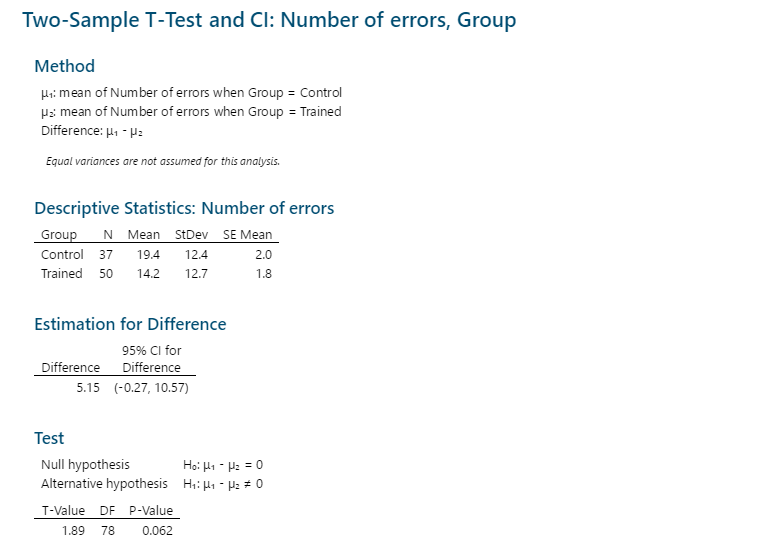
Minitab 18
The output from Minitab 18 is very clearly labelled and some rounding has already been done.

R
The output from the t-test command in R is shown below. Often the results provided by R need to be rounded. Note that there are some things missing that we need for the summary table:
- the group standard deviations, and
- the estimated difference in means.

You will need to use another function to obtain the group standard deviations, and you can get the difference in means as well, as shown below. However, the failure to provide this information is a poor oversight in the output of the t-test.
